How does MarkSim work?

General Circulation Models (GCMs) use columns of atmosphere covering about 200 by 300 km at ground level. So they do not simulate the weather on the ground at a particular place very accurately. To get back to what is expected in detail, we have to use downscaling. The mean deviation from the baseline for each atmospheric column (pixel) is re-evaluated to take into account the ground terrain and the characteristics of the expected weather.

This is often done with statistical downscaling, which uses the output of the GCM to compute a statistical relationship with existing meteorological data from a met station. That is then used to scale the results of the GCM to that of the station. This won't work on the global scale that we've used for MarkSimGCM simply because there are not enough met stations in the world.

There are two aspects to downscaling: one is to interpolate the results of the GCM spatially; and the other is to ensure that the results are relevant to the local climate. The spatial downscaling is the easiest part. This is usually done with a convolution algorithm — in our case it is a bicubic interpolation using the 16 points closest on a 1 degree grid.

Wilby et al. (2009) called this 'unintelligent downscaling' and we would agree, if this were all that we were doing. Our algorithm is based on the well-tried weather simulator MarkSim.

MarkSim is a weather generator that uses 720 classes of weather, worldwide, to calculate the coefficients of a third order Markov rainfall generator. This constitutes 'stochastic downscaling' as it fits a Markov model to the GCM output and uses it to generate weather data for the site indicated.

The third weapon in MarkSimGCM is built into the weather typing in the clustering process. The 720 classes of world weather define each set of regression equations that MarkSim uses to determine the coefficients for the modelling process. When a climate changes, such that it no longer applies to the original class, then the whole regression structure changes.

This means that a changing climate will be modelled by the one most like it in the real world. The only drawback is that the system cannot model completely new climates except by extrapolation of the regression models from the nearest cluster. But then we are still to see a new climate in sufficient detail to fit the model to it and GCM results are not precise enough to do this for the future. In the meantime, we will have to wait.

If you want to read about the application in more detail, see Jones & Thornton (2013). This documents the last version of the software. It is hoped that at some stage it will be updated. To see specific details that may be different follow the links on the ‘How to use MarkSimGCM’ page.

Jones, P. G. and Thornton, P. K. (2013) Generating downscaled weather data from a suite of climate models for agricultural modelling applications. Agric. Systems. 114 (2013) 1-5

Wilby R.L., Troni J., Biot Y., Tedd L., Hewitson B.C., Smith D.M. and Sutton R.T., 2009. A review of climate risk information for adaptation and development planning. Int. J. Climatol. 29, 1193-1215.


17 GCMs available in MarkSimGCM


Model

Institution

Resolution,

Lat x Long ¡

Reference

1

BCC-CSM 1.1 

Beijing Climate Center, China Meteorological Administration

2.8125 x 2.8125

Wu T (2012).  A Mass-Flux Cumulus Parameterization Scheme for Largescale Models: Description and Test with Observations. Clim. Dynam. 38, 725–744

2

BCC-CSM 1.1(m)

Beijing Climate Center, China Meteorological Administration

2.8125 x 2.8125

Wu T (2012).  A Mass-Flux Cumulus Parameterization Scheme for Largescale Models: Description and Test with Observations. Clim. Dynam. 38, 725–744

3

CSIRO-Mk3.6.0

Commonwealth Scientific and Industrial Research Organisation and the Queensland Climate Change Centre of Excellence

1.875 x 1.875

Collier MA et al. (2011) The CSIROMk3.6.0 Atmosphere-Ocean GCM: participation in CMIP5 and data publication. MODSIM 2011, Perth, 12–16 December 2011

4

FIO-ESM

The First Institute of Oceanography, SOA, China

2.812 x 2.812

Song Z, Qiao F, Song Y (2012). Response of the equatorial basin-wide SST to wave mixing in a climate model: An amendment to tropical bias, J. Geophys. Res., 117, C00J26

5

GFDL-CM3 

Geophysical Fluid Dynamics Laboratory

2.0 x 2.5

Donner LJ et al. (2011). The dynamical core, physical parameterizations, and basic simulation characteristics of the atmospheric component AM3 of the GFDL Global Coupled Model CM3. Journal of Climate, 24(13).

6

GFDL-ESM2G 

Geophysical Fluid Dynamics Laboratory

2.0 x 2.5

Dunne JP et al. (2012). GFDLÕs ESM2 Global Coupled Climate–Carbon Earth System Models. Part I: Physical Formulation and Baseline Simulation Characteristics. J. Climate, 25, 6646–6665.

7

GFDL-ESM2M

Geophysical Fluid Dynamics Laboratory

2.0 x 2.5

Dunne JP et al. (2012). GFDLÕs ESM2 Global Coupled Climate–Carbon Earth System Models. Part I: Physical Formulation and Baseline Simulation Characteristics. J. Climate, 25, 6646–6665.

8

GISS-E2-H

NASA Goddard Institute for Space Studies

2.0 x 2.5

Schmidt GA et al. (2006).  Present day atmospheric simulations using GISS ModelE: Comparison to in-situ, satellite and reanalysis data. J. Climate 19, 153-192.

9

GISS-E2-R

NASA Goddard Institute for Space Studies

2.0 x 2.5

Schmidt GA et al. (2006).  Present day atmospheric simulations using GISS ModelE: Comparison to in-situ, satellite and reanalysis data. J. Climate 19, 153-192.

10

HadGEM2-ES

Met Office Hadley Centre

1.2414 x 1.875

Collins WJ et al. (2011). Development and evaluation of an Earth-System model-HadGEM2. GMD 4(4):1051–1075.

11

IPSL-CM5A-LR 

Institut Pierre-Simon Laplace

1.875 x 3.75

Dufresne JL et al. (2013). Climate change projections using the IPSL-CM5 Earth System Model: from CMIP3 to CMIP5. Climate Dynamics, 1-43.

12

IPSL-CM5A-MR 

Institut Pierre-Simon Laplace

1.2587 x 2.5

Dufresne JL et al. (2013). Climate change projections using the IPSL-CM5 Earth System Model: from CMIP3 to CMIP5. Climate Dynamics, 1-43.

13

MIROC-ESM 

Atmosphere and Ocean Research Institute (The University of Tokyo), National Institute for Environmental Studies, and Japan Agency for Marine-Earth Science and Technology

2.8125 x 2.8125

Watanabe S et al. (2011). MIROC-ESM2010: model description and basic results of CMIP5-20c3m experiments. Geoscientific Model Development 4 (4), 845–872.

14

MIROC-ESM-CHEM

Atmosphere and Ocean Research Institute (The University of Tokyo), National Institute for Environmental Studies, and Japan Agency for Marine-Earth Science and Technology

2.8125 x 2.8125

Watanabe S et al. (2011). MIROC-ESM2010: model description and basic results of CMIP5-20c3m experiments. Geoscientific Model Development 4 (4), 845–872.

15

MIROC5 

Japan Agency for Marine-Earth Science and Technology, Atmosphere and Ocean Research Institute (The University of Tokyo), and National Institute for Environmental Studies

1.4063 x 1.4063

Watanabe M et al. (2010). Improved Climate Simulation by MIROC5: Mean States, Variability, and Climate Sensitivity. J. Climate, 23, 6312–6335.


16

MRI-CGCM3

Meteorological Research Institute

1.125 x 1.125

Yukimoto S (2012).  A new global climate model of Meteorological Research Institute: MRI-CGCM3 – Model description and basic performance. J. Meteorol. Soc. Jpn., 90a, 23–64

17

NorESM1-M 

Norwegian Climate Centre

1.875 x 2.5

Kirkevag A, Iversen T, Seland O, Debernard JB, Storelvmo T, Kristjansson JE (2008) Aerosol-cloud-climate interactions in the climate model CAM-Oslo.Tellus A 60(3):492–512.

Seland O, Iversen T, Kirkevag A, Storelvmo T (2008). Aerosol-climate interactions in the CAM-Oslo atmospheric GCM and investigation of associated basic shortcomings. Tellus A 60(3):459–491.


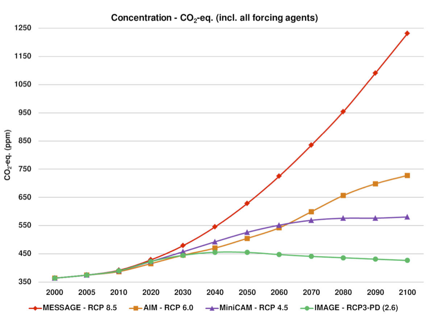
Representative Concentration Pathways (RCP)

These are the standardised set of future greenhouse gas emissions used by the General Circulation Models for the IPCC 5th approximation (CMIP5)

https://en.wikipedia.org/wiki/Representative_Concentration_Pathways

They integrate various future scenarios for CO2, Methane, Nitrous oxide, Fluorinated hydrcarbons and Ozone. Models were used to calculate the CO2 equivalent of the concentrations of these gasses under different future emission scenarios, taking into account their individual forcing values and lifetimes in the atmosphere.


Statistical average

A common way to represent the deviation from the baseline created by a GCM is to take a time slice off GCM data, often 10 years before and 10 years after the desired year. However this limits the number of years that can be represented as you’ve used 20 years to estimate one year. It would be possible to use a running mean of the 20 years, but this still limits to 10 years after the start of the data and 10 years before the end of the data. It also results in exceedingly large datasets.

We have found that in almost all cases, for all models, RCPs and pixels, fitting a fourth order regression through the deviations from baseline yields an error mean square indistinguishable from the historic baseline variance. The regressions are fitted through the origin at a notional point midway through the historic baseline data. This constrains the early years.

The result is an estimated deviation for any given year with an error term that uses all of the available data and so is actually better than a running mean. If the world is represented in 1 degree pixels, all the models and RCPs can be contained in a dataset that is only 2Gb which manageable for MarkSimGCM.

To interpolate the deviation to the exact point that you have selected we use a bicubic convolution algorithm. This fits a two dimensional cubic interpolation to the adjacent 16 points on the grid. This is not Thin Plate Smoothing (Laplacian splines) as the derivative is not conserved when the interpolation window shifts, but it is a continuous function and there are no steps in the surface. It is considerably faster than thin plate smoothing.


MarkSim CLX file

At present MarkSim uses an internal structure called CLX to hold the derived parameters for a model run. This structure also keeps track of the base climate data and the rotation of the record. In the original CD version of MarkSim a version of this was produced as an interim file. It is proposed to incorporate a version of the CLX interpretation code directly into DSSAT and so we must go back to the production of an actual CLX file. This section briefly describes the format of a CLX file.

Example file:

* GCMs included in ensemble
*        CSIRO-Mk3.6.0
*        HadGEM2-ES
*        IPSL-CM5A-LR
*        IPSL-CM5A-MR
*        MIROC5
*        NorESM1-M
* Year 2090
* Representative Concentration Pathway rcp8.5
CLXname        Lat        Long        Elev
Y_Waen        52.733     -3.950       95
Correlation Matrix, ordered by phase angle
7    1.000
8    0.247    1.000
9    0.133    0.115    1.000
10   0.010    0.090    0.078    1.000
11   0.057    0.100    0.092    0.010    1.000
12   0.025   -0.144   -0.022    0.038    0.048    1.000
1    0.044   -0.059   -0.012    0.050    0.030    0.072    1.000
2    0.076    0.024    0.114    0.086    0.083   -0.124    0.120    1.000
3    0.154    0.027   -0.012    0.058    0.070    0.095    0.081    0.127    1.000
4    0.021    0.010    0.070    0.001    0.115    0.113    0.106    0.073    0.185    1.000
5    0.047   -0.098   -0.052   -0.115    0.064   -0.033    0.071   -0.013    0.054    0.217    1.000
6    0.143    0.028    0.082   -0.022    0.108    0.033    0.106    0.036    0.012    0.131    0.047    1.000
Month Av    P    Beta Raindays S.E.
7    7.2 0.444 -0.964 0.321 0.25085
8    8.4 0.464 -0.887 0.371 0.24530
9    7.5 0.497 -0.768 0.452 0.23999
10   7.9 0.578 -0.572 0.590 0.23843
11  10.7 0.628 -0.745 0.468 0.24210
12  10.6 0.632 -0.727 0.481 0.24477
1    8.5 0.538 -0.836 0.405 0.24887
2    6.0 0.520 -0.653 0.534 0.24696
3    6.3 0.505 -0.698 0.502 0.24339
4    5.4 0.458 -0.886 0.371 0.24714
5    6.1 0.450 -0.921 0.348 0.24637
6    6.0 0.435 -1.010 0.293 0.25378
Lag parameters, rainfall 1.0148 0.3136 0.0728
Stations in Cluster                21
Cluster number                    423
Distance to cluster centre     1.7107
Phase angle of rotation        3.4280
             Jan    Feb    Mar    Apr    May    Jun    Jul    Aug    Sep    Oct    Nov    Dec  
rainfall   132.8   93.8  104.3   77.8   61.2   60.0   57.4   81.9   90.6  122.0  147.1  157.9
Max Temp     9.5    9.9   11.8   14.6   18.6   22.1   24.7   24.4   22.0   17.7   13.1   10.7
Min Temp     5.4    5.3   6.4     8.0   11.1   14.3   17.1   17.3   15.2   11.6    8.0    6.7
Radiation    1.0    1.8   3.7     5.9    9.7   12.8   15.5   15.1   11.3    6.5    2.1    1.2

IT IS NOT ADVISABLE TO CHANGE ANY FIELD IN A CLX FILE AS MANY ARE INTERRELATED AND CHANGES COULD HAVE UNFORESEEN EFFECTS

The records preceded by an asterisk are descriptive of the origin of the data. There will be a variable number of these depending on the selection. I.E, present day climate, one GCM, a selection of GCMs, or all 17 GCMs in an ensemble.    All other records are mandatory and fixed format.

The correlation matrix is shown rotated to the nearest month and only the lower triangle is printed. The markov rainfall monthly parameters are shown in the columns that follow. The values are the precise rotated values; the month indicated is the nearest and shown as a guide.

The lag parameters are the probit values added to Beta for rain falling on days –1, -2 and –3. The number of stations in the cluster refers to the original calibration stations that went into the assigned cluster to form the parameter regression models. The cluster distance shows the distance from the centre of the assigned cluster in standardized 36-dimensional space. The rotation angle is in radians, it is the angle subtracted from the first phase angle of the record to normalise it in the meteorological year. This allows for comparison of station records from different parts of the globe.

The monthly climate data in the last four records of the file are re-rotated to true monthly values.


ILRI © 2010 - 2014. Terms of Use. Developed by egiron